
Table of Contents
(Long) introduction
Recently, I had to copy the skin weights of an object on another object. The typical exemple is when you have some cloth on a skin and you want to copy the cloth weights on the skin.

As usual, the modeling is not from me, but from Claire Blustin, best modeler in the world!
Considering the fact I skinned some parts of the skin already (the fingers), I didn't want to loose what I had already by copying the cloth on top of it. I know maya's native copy skin can work on components, i didn't want to select manually all the vertices i wanted to target (especially at the very beginning of a production, knowing that i'd have to do it again and again!).
Anyway... so I wanted to do a little tool to select automatically all the vertices on the skin that are at less than x units of distance from the closest point on the cloth. Plus it'll always be useful for something else...
Maya gives us the tools to do it already! Let's use some getClosestPoint(), and it should do the trick and let me some time to chill on youtube instead of painfully select all my vertices manually!
  from maya.OpenMaya import *
  from fn import fApi
  def getClosestVertices(src, dst, tol=0.1):
      '''
      With a given source mesh and destination mesh,
      will select all the vertices of the destination mesh that are
      at a given distance of the closest point on the source mesh
      (the given distance being 'tol' argument)
      '''
      # just returns an MObject, based on the given string
      mSrc = fApi.nameToMObject(src)[0]
      mDst = fApi.nameToMObject(dst)[0]
      # i get a dagPath because if we give just the
      # mobject to the fn set or the iterator,
      # obviously, we can't work in world space.
      dagSrc = MDagPath()
      dagDst = MDagPath()
      MDagPath.getAPathTo(mSrc, dagSrc)
      MDagPath.getAPathTo(mDst, dagDst)

      fnSrc = MFnMesh(dagSrc)
      it = MItMeshVertex(dagDst)

      includedVertices = []
      while not it.isDone():
          closestPoint = MPoint()
          currPoint = it.position(MSpace.kWorld)
          fnSrc.getClosestPoint(currPoint, closestPoint, MSpace.kWorld)
          v = currPoint - closestPoint
          if v.length() < tol:
              includedVertices.append(it.index())
          it.next()
      return includedVertices
Not really clean, but that'll do the job. I'll do a pass of cleaning later!
So here we go! I run my code, and... maya crash? No, the expected result, but it took more than 20 fucking seconds to process!
Patience has never been my best quality, no way to keep something so long. And at this point, I already know what's causing the process to be so heavy! Like every time we use maya commands over pure code, we use a wrapper (and in this case, a python wrapper of a c++ wrapper of the core of maya! And who knows which algorithm the core is using...).
Then I remembered a discussion I had with my former HOD, about something called 'kd-trees', used to optimize drastically proximity operations in an n-dimentional space. Time to investigate a bit further!
As it seems to be a huge field of research (and brand new to me!), I will focus here on the theory, and won't go into details. For a python implementation, i can share mine if you want (just ask me on email), or a quick google search will bring you on the repo of someone who did it already. I didn't test this out, though. Finally, numpy/scipy come with some tools to do it too, i think. But my point is that you won't find here every bits and bobs that you can just copy/paste to have something working.
What is a k-d tree
Definition and meaning
As usual, behind this mysterious name, the idea is not that difficult. Of course,
Before going into too much detail, I can submit my own definition, probably not super accurate, but at least it uses simple words!
Example, using a 2-d tree
Let's see now the structure of k-d tree in detail! We'll work with only 2 dimensions at first, to keep things simple.
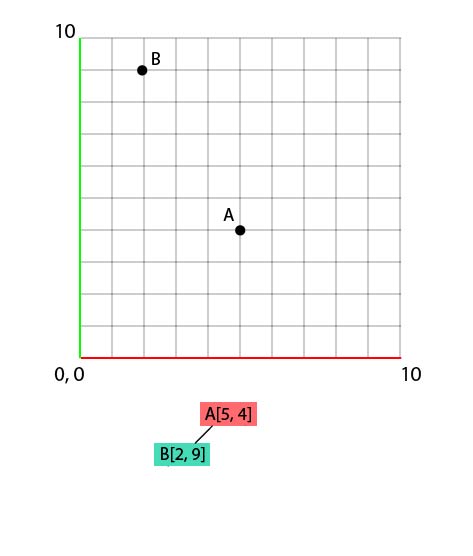
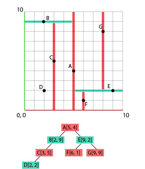
Let's assume the following set of coords :
- A[5, 4]
- B[2, 9]
- C[3, 5]
- D[2, 2]
- E[9, 2]
- F[6, 1]
- G[9, 9]
We'll generate, from this set, a k-d tree, and put those points on a 2d grid at the same time. Let's start with A. Nothing crazy here:

While doing that, let's also add A at the bottom, under the grid. This first 'node', below the grid, will be our 'root' node for this tree. Then, we populate information just like any type of tree. Each node has children, each child has other children, and so on and so forth! In the case of a k-d tree, there are always 2 children, one on the left, one on the right. Now, how to define if a child should take place on the right or the left ? By comparing the position values, dimension by dimension.
To set B, we'll compare his x value with the x value of A, like so :
- B.x < A.x because
- 2 < 5
So our B point will take place on the left of A, in the tree (and on the grid as well, obviously, as we were comparing the 'x' value. But I do hope that you know how to put a point on a grid if you have its coords. ^^)!
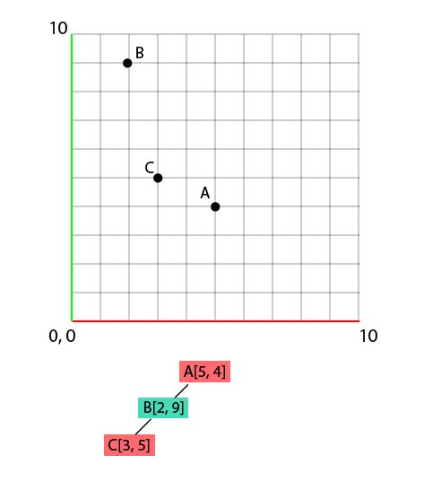
Let's move on to C[3, 5].
- We'll compare first the value C.x (3) against A.x (5), to deduce that C will go to the left.
- Then we'll compare C.y to B.y. In this case, C.y is smaller than B.y, therefore our C will go to the left of B.
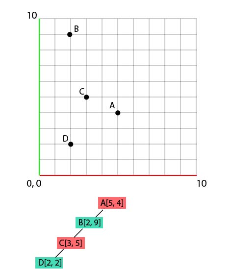
Now D[2, 2].
- D.x compared to A.x -> 2 compared to 5 : left
- D.y compared to B.y -> 2 compared to 9 : left again...
- D.x compared to C.x -> 2 compared to 3 : and left again!
And let's continue with the same logic to end up with this result :
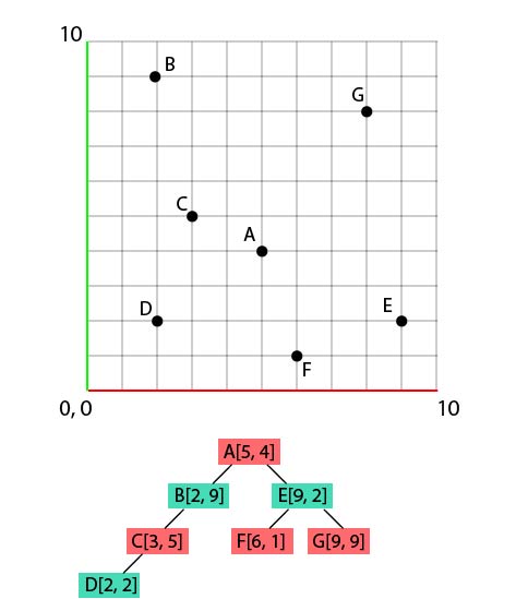
Done, our tree is ready!
The KEY thing to understand is that we swap axis between each comparison, and we work every time on 1 and only 1 axis! To understand better the consequences of this workflow in a 3d space (or in a 2d space, in our case), let's draw some extra markers!
Starting with A, what we actually do is that we put its children regarding their X value. In other words, we split our grid into 2 parts, in perpendiculary axis (once again, in 2d, it's easy, it has to be the 'other' axis, Y here). If the x value of the child is smaller than its parent's x value, the child goes to the left, otherwise it goes to the right :

Then, we split again the grid in 2, but this time, horizontally (i.e. perpendicular to Y axis), in one and the other half, based on the next point.

By doing that recursively, we end up with a super split space, in which it becomes much faster and easier to navigate. If we simplify the idea : you compare your first point only in 1 dimension instead of 3, and from that result, you can already eliminate half of the points! You know the closest point won't be here! So you decimate elements of the graph much faster, by removing half of what remains on every iteration!)
Using a k-d tree in 3 dimensions
Possible k-dimensions implementation
What I submit here is a possible implementation of a method to generate a k-d tree. In order to keep things as simple as possible, i removed a huge part of what would be necessary to have a robust code. Therefore, this method on its own is not usable. Take it more as a pseudo-code than as a ready-to-use function. For something that you can use with no modification (but obviously much longer and complex), I suggest that you check out the github link I gave in the introduction
  def buildTree(datas, depth=0):
      ''' Builds a tree made of KdNodes. The tree is ran recursively '''
      # in order to swich axis at each iteration, we get the modulo of
      # depth % number of dimensions, so axis will be 0%3=0 (x),
      # 1%3(y), 2%3(z), and will come back to 0 (3%3), 1 (4%3), and so on)
      axis = depth % dimensions

      # then, we'll sort our list of arrays, based on the dimension we want
      # for example, if we sort A(1, 4), B(2, 2) and C(5, 1) by y
      # (using key=lambda pt: pt[1]), we'll get C, B, A
      datas.sort(key=lambda pt: pt[axis])
      # the mid point for this dimension will be the middle-th element
      # of the list (we use // because we want an index (i.e. int), not
      # a float, obviously)
      midPointIdx = len(datas)//2

      # so all we have to do is to split this list, create a node from
      # the current mid value (the Node class can store the left and
      # right child, for example),
      # and run buildTree again with the remaining 2 arrays.
      currentPoint = datas[midPointIdx][0]
      left = buildTree(datas[:midPointIdx], depth+1)
      right = buildTree(datas[midPointIdx+1:], depth+1)
      currentNode = KdTree.KdNode(currentPoint, left, right)

      return currentNode
Reading the values from the tree
In a way, we could compare this process to any other compression / decompression module we're used to, such as cPickle, configParser or json, that we frequently use in maya. When creating the tree, we kind of 'json.dump()' our point array. But to take advantage of it, one would need to 'json.load()' it, i.e. uncompress it, so to speak.
Unfortunately, we're entering here in something muuuuuuuch more complex, which is a field of expertise on its own, and an important challenge in modern computer graphics, from what I understood. Just like every low level algorithm (such as decomposition LU, or even worst, boolean algebra (I recommand this amazing book, if you're interested in this topic!)), it's the starting point of massive calculations (if you save 0.1s on an operation that you'll perform 50 000, you can easily see how significant would be even the smaller improvement on the base code!). Therefore, it opens the door to much more complex (and fun) tools, such as a proximity maps!
So I won't go into too much detail on that, firstly because I'm miles away from a good understanding, and secondly because I wouldn't even know where to start. The few last days I spent in researches showed me that there are a few different implementations, and I definetly don't have time (and probably knowledge ^^) to benchmark all of them!
Now why is that so efficient? The general idea, as we said, is that we can isolate super quickly the closest element using a boolean logic. Regarding the tree hierarchy, and with a given point P, we'll compare P.x with the root.x. If greater, we look for the nearest point in the right part, otherwise in the left part. it's 0 or 1, true or false, left or right. Same thing with the next level, and so on. The limitation, of course, is that unlike the getClosestPoint(), you'll get the closest vertex, not the closest point. The heavier the mesh is, the smaller the error will be, and the faster the processing will be, compared to the getClosestPoint() method. But in the case of a super low poly mesh, obviously, it'd probably be better to use the getClosestPoint instead, as the time would't be a problem.
I'd advice, if you want to go further, to have a look at the siggraph papers, or some other technical papers you can find on the internet. For my implementation, I sticked to this paper, more because it was easy than because of a real choice. The dudes talk about computer science, so I assumed it was pretty similar to my needs and requirements. If you're really interested, do not hesitate to let me know in the comments, and I'll try to debunk the concept, at least for the implementation i choosed!
The interest, ultimately, is to be able to query very quickly the closest point, and therefore, the distance that separates this closest point from the query point, the exact position of this vertex in world space, the index of this vertex, etc... Considering that there is almost no calculation, just a particular method of sorting huge arrays, you can attach any info you want against each element of your array!
Conclusion
So all those stuff brought us far from the initial problem! But to motivate you looking into k-d trees, i replaced the call to getClosestPoint() by my implementation of a k-d tree, and go from 8.62844705582s down to 1.25752019882s of evaluation (600% improvement, booom!). And I'm sure i can optimize it, and this is just pure python! Imagine the result with a decent c++ version!
I hope that this small introduction to k-d trees will motivate you looking at it. If you want to know more (in particular on how to get the results back), do not hesitate to let me know in the comments. On my side, I must confess that gives me tons of ideas of tools! So time to work!