What is clustering?

Clustering is a method with a broad range of applications, from data science to image compression and 3D.

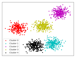
In a nutshell, the whole point of clustering is to use your machine to do something ridiculously basic for a human: given a point cloud, how can we group them in a way that makes sense (e.g. by proximity)

This is the first image I found on google image to illustrate. You can see 5 different clusters, which, again, is obvious for a human, but not so much for a machine

This tutorial is not purely related to Maya (as in we're not gonna open maya nor produce anything usable straight out of the box), but you might find some nice uses for clustering in various problems (e.g. smooth skinning decomposition with rigid bones). Again, we're here to understand and have fun with clusters, not to do something someone will pay you for =p

You can find a snippet of code at the end of this tutorial that will summarize everything we're gonna see here. Make sure to install all the required dependencies if you want to follow along

Representing an image in 3d

We're gonna focus on how to use clustering for image compression (told you, wide range of applications!). Of course, this is more of a 90's algorithm for image compression, but it has the advantage of being trivial to understand. I'm gonna create a ridiculously simple image, and the goal is gonna be for us to compress it, by reducing the number of colors; basically, instead of having 16 millions of colors, we want to have only a few of them (3, 5, maybe 7 if we want to go crazy!); of course, less data to store = lighter image.

here is our simple image

Now let's consider this image pixel by pixel. Each pixel is made of 3 numbers, running from 0 to 255

Each pixel value being stored on an octet, i.e. 8 bits, it can vary between 1 and 2⁸,
that is, 1-256, or, in computer science, 0-255

For an arbitrary pixel, located on the grid of pixels at 6 vertically and 4 horizontally (from top left corner), the rgb color is 25 (red), 203 (green), 254 (blue). Now let's bring those values between 0 and 1 (what we call "normalizing"), by dividing them by 255. We get rgb(0.098, 0.796, 0.996).

Convert rgb into xyz

Ok, we know the rgb value of this pixel. Now why do we have to keep it as a color? Instead, we could think of this pixel as a point, in a 3d space:

red color would be its X position
green would be Y
and blue would be Z

Why not expanding this logic to every pixel in our image, and plot the result? We should end up with a point cloud, corresponding to the color repartition

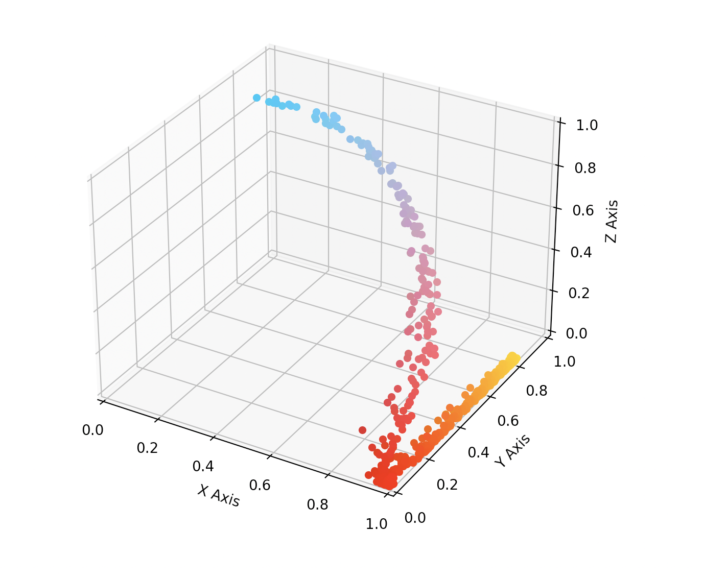
Point cloud representing our 2d colored image

As you can see, every pixel is placed in a 3d space based on its color. The points are colored based on their original color

Furthermore, you can clearly see that red and orange points are pushed along the Y axis, depending on their orange-ness. And indeed, red+green=yellow

Now, let's make some magic! Implementing a clustering algorithm is obviously beyond the scope of this tutorial and people smarter than us already did it for us! So we're gonna use the existing ones. Here, we're using KMeans, from sklearn.cluster (sklearn is a great machine learning library I encourage you to try). KMeans takes the number of clusters requested as an argument. To make the demonstration obvious, we'll reduce the number of clusters to 3. Now let's plot the point cloud again, but this time, we will color each pixel/point based on the average of the cluster to which it belongs.

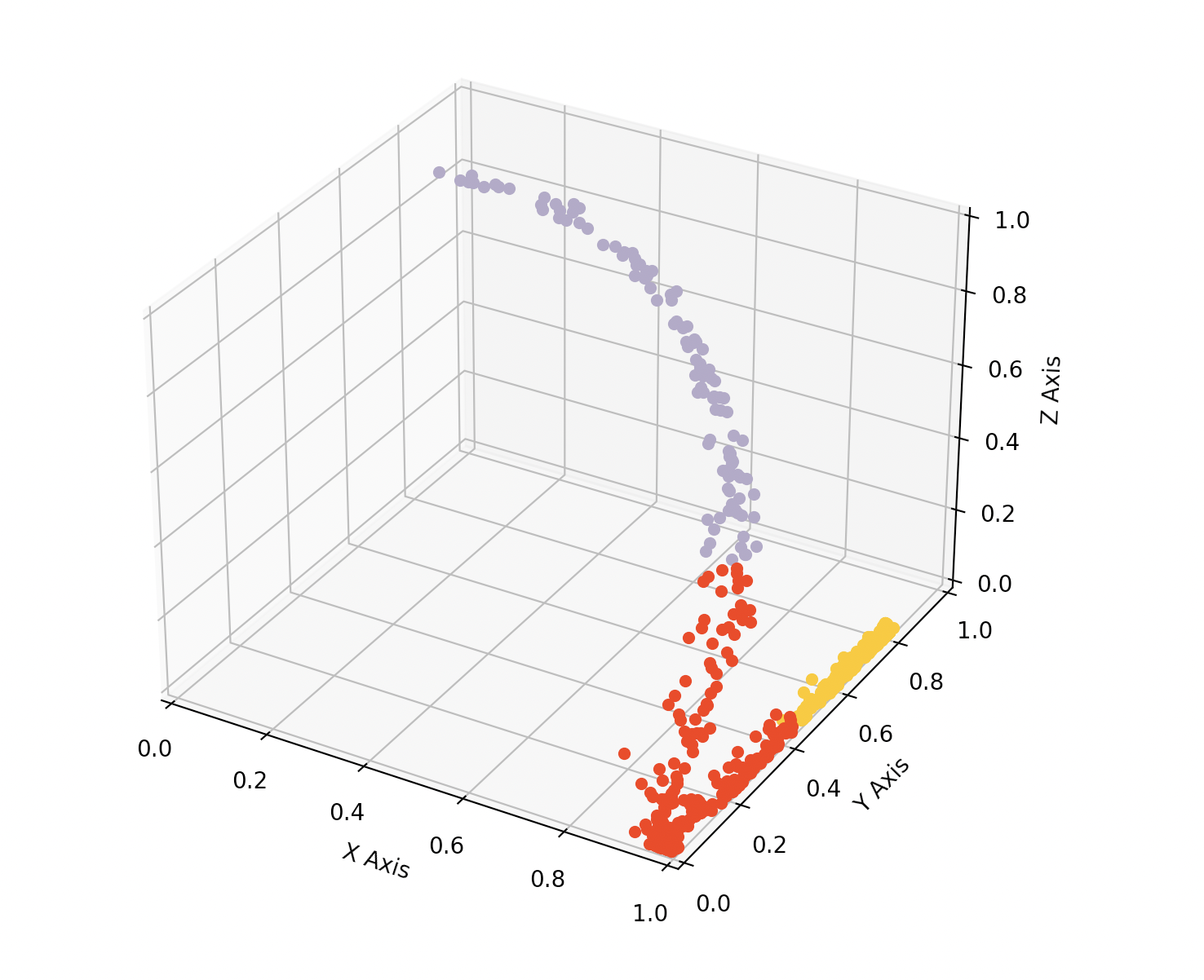
Here, we can clearly see the 3 clusters

As you can see, KMeans gave us 3 clusters that we can clearly see on the 3d view.

Now that we know each pixel / point is bound to a cluster, let's rebuild the original image to see how it looks like.

Voila! Our compressed image!

We reduced the original image with god knows how many colors to something much lighter with only 3 colors. Of course, this is a bit too much, and the data loss is too important. Let's try again but this time we'll increase a little bit the number of clusters. Let's put it to 16

16 colors only

Now we're getting something better! Only 16 colors (which is clearly nothing, compared to the initial 16 millions). Again, there is a data loss, but also a massive gain in weight. And doesn't it remind you of those images we had back in the 90's? =]

Code

Finally, here is a snippet of code to reproduce everything we did here. Make sure you have all the required libraries, as some of them don't come with python by default.

from mpl_toolkits.mplot3d import Axes3D
import matplotlib.pyplot as plt
import numpy as np
import sys
from skimage import io
from sklearn.cluster import KMeans

from PIL import Image

def read_image():
    im = Image.open('/tmp/img.jpg')
    pix = im.load()
    pixel_values = np.array(im.getdata())
    pixel_values = pixel_values/255
    return pixel_values


def plot_colors_as_xyz(pixel_values, colors, fig):
    ax = fig.add_subplot(111, projection='3d')

    for i, pixel in enumerate(pixel_values):
        ax.scatter(pixel[0], pixel[1], pixel[2], color=colors[i])

    ax.set_xlabel('X Label')
    ax.set_ylabel('Y Label')
    ax.set_zlabel('Z Label')
    ax.set_xlim(0, 1)
    ax.set_ylim(0, 1)
    ax.set_zlim(0, 1)



image = io.imread('/tmp/img.jpg')
# io.imshow(image)
# io.show()

#Dimension of the original image
rows = image.shape[0]
cols = image.shape[1]

#Flatten the image
image = image.reshape(rows*cols, 3)

fig = plt.figure()
# plot_colors_as_xyz(image/255, image/255, fig)

kmeans = KMeans(n_clusters=16)
kmeans.fit(image)

compressed_image = kmeans.cluster_centers_[kmeans.labels_]
compressed_image = np.clip(compressed_image.astype('uint8'), 0, 255)

#Reshape the image to original dimension
plot_colors_as_xyz(image/255, compressed_image/255, fig)
compressed_image = compressed_image.reshape(rows, cols, 3)
#Save and display output image
io.imsave('/tmp/img.png', compressed_image)
# io.imshow(compressed_image)
# io.show()
plt.show()

Table of Contents

What is clustering?

Representing an image in 3d

Convert rgb into xyz

Code